
In today’s data-driven world, organizations constantly collect vast amounts of data. However, not all data is created equal, and datasets may contain unexpected or unusual patterns or data points, known as anomalies or outliers. These anomalies can provide valuable insights into data quality, potential risks, and operational efficiency. However, detecting anomalies can be challenging, especially when dealing with large and complex datasets.
This is where anomaly detection techniques come into play. Anomaly detection is the process of intelligently identifying unusual or unexpected patterns or data points in a dataset. By leveraging the top anomaly detection techniques, organizations can gain insights into their data, prevent fraud, and improve their model performance. Whether you are working in finance, cybersecurity, manufacturing, or healthcare, anomaly detection is a crucial tool that can help you gain insights into your data and make better decisions.
What is Anomaly Detection and Its Role in Data Quality?
Anomaly detection refers to identifying unusual or unexpected patterns or data points in a dataset. It plays a crucial role in ensuring data quality. Data quality refers to the accuracy, completeness, and consistency of data. Poor data quality can lead to wasted resources since models must be re-trained on new and clean data.
To learn about the 5 most essential data cleaning techniques, follow this article.
Anomaly detection can help identify potential errors or inconsistencies in data, allowing organizations to address these issues and improve data quality. For example, anomaly detection is used in the finance industry to identify unusual or unexpected patterns in financial transactions. These patterns indicate potential fraud, which can be addressed to improve data quality and protect financial assets.
Top Anomaly Detection Techniques
Several different methods exist for detecting anomalies in a dataset utilizing different features. Let’s dive deeper into the following five most popular techniques for anomaly detection..
Statistical Methods
Statistical methods for anomaly detection are based on identifying data points that deviate from expected statistical distributions or patterns. These methods are often simple to implement and can be useful when the dataset is small or when the data is expected to follow a specific statistical distribution. Some common statistical methods for anomaly detection include the percentile and interquartile range (IQR) methods.
Percentile method
The percentile method is based on identifying data points that fall outside a specific percentile range. This method considers data points that fall outside the specified percentile range anomalies.
Here’s an example code snippet demonstrating the percentile anomaly detection method using Python.
import numpy as np

# Generate a random dataset
data = np.random.normal(0, 1, 1000)

# Define the percentile range for anomaly detection
percentile_range = (1, 99)

# Identify the values at the specified percentiles
percentiles = np.percentile(data, percentile_range)

# Identify anomalies
anomalies = np.where((data < percentiles[0]) | (data > percentiles[1]))

# Print the indices of the anomalies
print("Anomalies:", anomalies)
Interquartile range (IQR) method
The interquartile range (IQR) method is based on the range between the first and third quartiles of the dataset. In this method, data points that fall outside a certain IQR range are considered anomalies.
In Python, this is implemented as the following.
import numpy as np

# Generate a random dataset
data = np.random.normal(0, 1, 1000)

# Calculate the first and third quartiles of the dataset
q1, q3 = np.percentile(data, [25, 75])

# Calculate the interquartile range of the dataset
iqr = q3 - q1

# Define the IQR range for anomaly detection
iqr_range = (q1 - 1.5 * iqr, q3 + 1.5 * iqr)

# Identify anomalies
anomalies = np.where((data < iqr_range[0]) | (data > iqr_range[1]))

# Print the indices of the anomalies
print("Anomalies:", anomalies)
Clustering-Based Methods
Clustering-based methods for anomaly detection involve grouping similar data points into clusters and then identifying data points that are not part of any cluster or belong to a cluster significantly different from the others. These methods work well for detecting local anomalies which occur in a specific region of the dataset. Clustering-based methods can also identify global anomalies which occur across the entire dataset.
K-Means Clustering
One popular clustering-based method for anomaly detection is the k-means clustering algorithm. The k-means algorithm groups data points into “k” clusters based on their similarity, which can be calculated by Euclidean distance in the feature space or other similar methods. Data points that do not fit well into any of the clusters or belong to a cluster with a significantly different distribution are considered anomalies.
Here is an example code snippet demonstrating the k-means clustering method for anomaly detection.
import numpy as np
from sklearn.cluster import KMeans

# Generate a random dataset
data = np.random.normal(0, 1, (1000, 2))

# Fit the k-means algorithm to the dataset
kmeans = KMeans(n_clusters=5).fit(data)

# Get the distances of each point to its nearest cluster
distances = kmeans.transform(data)
nearest_distances = np.min(distances, axis=1)

# Define a threshold for anomaly detection
threshold = np.percentile(nearest_distances, 95)

# Identify anomalies
anomalies = np.where(nearest_distances > threshold)

# Print the indices of the anomalies
print("Anomalies:", anomalies)
DBSCAN Clustering
Another clustering-based method for anomaly detection is the density-based spatial clustering of applications with noise (DBSCAN) algorithm. The DBSCAN algorithm groups data points into clusters based on their density. Data points not part of any cluster or belonging to a cluster with a significantly different density are considered anomalies.
import numpy as np
from sklearn.cluster import DBSCAN

# Generate a random dataset
data = np.random.normal(0, 1, (1000, 2))

# Fit the DBSCAN algorithm to the dataset
dbscan = DBSCAN(eps=0.5, min_samples=5).fit(data)

# Identify anomalies
anomalies = np.where(dbscan.labels_ == -1)

# Print the indices of the anomalies
print("Anomalies:", anomalies)
Machine Learning-Based Methods
Machine learning-based methods for anomaly detection involve using supervised or unsupervised machine learning algorithms to automatically identify anomalies in data without solely relying on traditional data statistics. These methods typically require a training dataset with both normal and anomalous data points to build a model that can identify anomalies in new data.
Supervised Methods
Supervised machine learning algorithms are trained on a labeled dataset that includes both normal and anomalous data points. The algorithm learns to classify new data points as either normal or anomalous based on the features of the data. The performance of the algorithm can be evaluated using metrics such as accuracy, precision, recall, and F1-score.
Support Vector Machines
SVM is a popular supervised machine learning algorithm for anomaly detection. They are effective in separating data points into two classes based on the features of the data. The algorithm learns to draw a boundary between the normal and anomalous data points in the feature space. Data points that fall outside this boundary are classified as anomalies.
import numpy as np
from sklearn.svm import OneClassSVM

# Generate a random dataset
data = np.random.normal(0, 1, (1000, 2))

# Train an One-Class SVM on the dataset
svm = OneClassSVM(gamma='auto').fit(data)

# Predict the anomaly scores for each data point
scores = svm.score_samples(data)

# Define a threshold for anomaly detection
threshold = np.percentile(scores, 5)

# Identify anomalies
anomalies = np.where(scores < threshold)

# Print the indices of the anomalies
print("Anomalies:", anomalies)
Confidence Learning
Confidence learning is a technique in machine learning where a model is trained to predict not only the class or label of a given input but also the confidence or certainty of its prediction. In other words, the model learns to assign a probability or score to each possible class, indicating how confident it is in its prediction.
This is particularly useful in anomaly detection, where identifying rare events or outliers is crucial. By using confidence learning, we can train a model to not only detect anomalies but also to estimate the likelihood or probability that a given input is anomalous.
Here is an example of implementing confidence learning in PyTorch.
import torch
import torch.nn as nn
import torch.optim as optim
from torch.utils.data import DataLoader, Dataset

class AnomalyDetector(nn.Module):
    def __init__(self):
        super(AnomalyDetector, self).__init__()
        self.encoder = nn.Sequential(
            nn.Linear(28*28, 128),
            nn.ReLU(),
            nn.Linear(128, 64),
            nn.ReLU(),
            nn.Linear(64, 32),
            nn.ReLU(),
            nn.Linear(32, 16),
            nn.ReLU(),
            nn.Linear(16, 8),
            nn.ReLU(),
            nn.Linear(8, 4),
        )
        self.decoder = nn.Sequential(
            nn.Linear(4, 8),
            nn.ReLU(),
            nn.Linear(8, 16),
            nn.ReLU(),
            nn.Linear(16, 32),
            nn.ReLU(),
            nn.Linear(32, 64),
            nn.ReLU(),
            nn.Linear(64, 128),
            nn.ReLU(),
            nn.Linear(128, 28*28),
            nn.Sigmoid(),
        )
        self.criterion = nn.MSELoss()

    def forward(self, x):
        z = self.encoder(x)
        x_hat = self.decoder(z)
        return x_hat, z

    def training_step(self, batch):
        x, _ = batch
        x_hat, z = self(x)
        loss = self.criterion(x_hat, x)
        return loss

    def validation_step(self, batch):
        x, _ = batch
        x_hat, z = self(x)
        loss = self.criterion(x_hat, x)
        return {'val_loss': loss}

    def validation_epoch_end(self, outputs):
        avg_loss = torch.stack([x['val_loss'] for x in outputs]).mean()
        return {'val_loss': avg_loss}

    def configure_optimizers(self):
        optimizer = optim.Adam(self.parameters(), lr=1e-3)
        return optimizer

class ConfidenceAnomalyDetector(AnomalyDetector):
    def __init__(self):
        super(ConfidenceAnomalyDetector, self).__init__()
        self.confidence_layer = nn.Sequential(
            nn.Linear(4, 2),
            nn.Softmax(dim=1)
        )

    def forward(self, x):
        z = self.encoder(x)
        x_hat = self.decoder(z)
        confidence = self.confidence_layer(z)
        return x_hat, z, confidence

class AnomalyDataset(Dataset):
    def __init__(self, X):
        self.X = torch.Tensor(X)

    def __len__(self):
        return len(self.X)

    def __getitem__(self, idx):
        x = self.X[idx]
        return x, 0

# train the model with confidence learning
model = ConfidenceAnomalyDetector()
train_dataset = AnomalyDataset(X_train)
train_dataloader = DataLoader(train_dataset, batch_size=128, shuffle=True)
val_dataset = AnomalyDataset(X_val)
val_dataloader = DataLoader(val_dataset, batch_size=128)
trainer = pl.Trainer(max_epochs=100, progress_bar_refresh_rate=10, gpus=1)
trainer.fit(model, train_dataloader, val_dataloader)

# detect anomalies with confidence scores
test_dataset = AnomalyDataset(X_test)
test_dataloader = DataLoader(test
_dataset, batch_size=128)
anomalies = []
for x in test_dataloader:
    score, is_anomaly = model(x.to(device))
    anomalies.extend(x[~is_anomaly.cpu().numpy()])

#plot the anomalies
anomalies = torch.stack(anomalies).cpu().numpy()
plt.plot(X_test, label='normal')
plt.scatter(np.arange(len(anomalies)), anomalies, label='anomaly', color='red')
plt.legend()
plt.show()
Unsupervised Methods
Unsupervised machine learning-based methods for anomaly detection involve training models on a dataset without any labels indicating the presence of anomalies. These models can then detect anomalies in new, unseen data.
One of the advantages of unsupervised machine learning-based methods for anomaly detection is that they can be used to detect previously unseen anomalies that were not present in the training data. However, because they do not use labeled data, it can be challenging to determine the severity or importance of the detected anomalies. One popular unsupervised method for anomaly detection is the isolation forest algorithm, which uses decision trees to isolate anomalies from the rest of the data.
Here’s an example of how to implement the isolation forest algorithm in Python using the scikit-learn library.
from sklearn.ensemble import IsolationForest
import numpy as np

# Generate some random data
X = np.random.normal(0, 0.1, size=(1000, 2))
X[:10] = np.random.normal(5, 0.5, size=(10, 2))

# Create and fit the isolation forest model
clf = IsolationForest(n_estimators=100, contamination=0.05, random_state=42)
clf.fit(X)

# Predict the anomalies
y_pred = clf.predict(X)

# Get the indices of the anomalies
anomaly_indices = np.where(y_pred == -1)[0]
Deep Learning-Based Methods
Deep Learning-based methods are also automatic anomaly detectors. Deep Learning itself is a subset of Machine Learning. However, Deep Learning models tend to be more complex, and they are automatic feature extractors and predictors, unlike Machine learning models that use handcrafted features.
Deep learning-based methods have shown great success in detecting anomalies in high-dimensional datasets. These methods rely on neural networks with multiple hidden layers to learn complex patterns in the data and identify anomalies based on deviations from these learned patterns. Autoencoders are famous for this.
Autoencoders are composed of two distinct parts- an encoder and a decoder. The encoder maps the input data to a lower-dimensional latent space representation, and the decoder reconstructs the original input from the latent space representation. When an anomaly is encountered, a trained autoencoder is less able to accurately reconstruct the input data, indicating the presence of an anomaly.
Here is an example of how to implement an autoencoder for anomaly detection on the MNIST dataset.
import torch
import torch.nn as nn
import torch.optim as optim
from torch.utils.data import DataLoader, Dataset

# Define the autoencoder architecture
class Autoencoder(nn.Module):
    def __init__(self):
        super(Autoencoder, self).__init__()
        self.encoder = nn.Sequential(
            nn.Linear(28 * 28, 128),
            nn.ReLU(),
            nn.Linear(128, 64),
            nn.ReLU(),
            nn.Linear(64, 12),
            nn.ReLU(),
            nn.Linear(12, 2),
        )
        self.decoder = nn.Sequential(
            nn.Linear(2, 12),
            nn.ReLU(),
            nn.Linear(12, 64),
            nn.ReLU(),
            nn.Linear(64, 128),
            nn.ReLU(),
            nn.Linear(128, 28 * 28),
            nn.Sigmoid(),
        )

    def forward(self, x):
        x = self.encoder(x)
        x = self.decoder(x)
        return x

# Define the dataset class
class MNISTDataset(Dataset):
    def __init__(self, data, targets):
        self.data = data
        self.targets = targets

    def __getitem__(self, index):
        x = self.data[index].flatten().float()
        y = self.targets[index]
        return x, y

    def __len__(self):
        return len(self.data)

# Load the MNIST dataset
train_data = torchvision.datasets.MNIST(root='./data', train=True, download=True, transform=torchvision.transforms.ToTensor())
test_data = torchvision.datasets.MNIST(root='./data', train=False, download=True, transform=torchvision.transforms.ToTensor())

train_loader = DataLoader(MNISTDataset(train_data.data, train_data.targets), batch_size=64, shuffle=True)
test_loader = DataLoader(MNISTDataset(test_data.data, test_data.targets), batch_size=64, shuffle=False)

# Define the autoencoder model and optimizer
autoencoder = Autoencoder()
optimizer = optim.Adam(autoencoder.parameters(), lr=0.001)

# Train the autoencoder
num_epochs = 10
for epoch in range(num_epochs):
    for data, _ in train_loader:
        data = data.view(data.size(0), -1)
        optimizer.zero_grad()
        recon_data = autoencoder(data)
        loss = nn.BCELoss()(recon_data, data)
        loss.backward()
        optimizer.step()
    print(f'Epoch [{epoch+1}/{num_epochs}], Loss: {loss.item():.4f}')

# Detect anomalies in the test set
anomaly_scores = []
for data, _ in test_loader:
    data = data.view(data.size(0), -1)
    recon_data = autoencoder(data)
    loss = nn.BCELoss(reduction='none')(recon_data, data)
    loss = loss.sum(dim=1)
    anomaly_scores += loss.tolist()

# Visualize the anomaly scores
import matplotlib.pyplot as plt

plt.hist(anomaly_scores, bins=50)
plt.xlabel('Anomaly Score')
plt.ylabel('Count')
plt.show()
Time Series-Based Methods
Time series-based methods are instrumental in detecting anomalies in sequential data where the order of the data points matters- for example, audio or video data. LSTM is one of the most popular techniques for anomaly detection in time-series data.
LSTM (Long Short-Term Memory) is a specialized type of recurrent neural network (RNN) designed to model long-term dependencies in time series data. Unlike traditional RNNs, LSTM incorporates a memory cell that can store information for a prolonged period, allowing it to handle sequences with long gaps between relevant events. This makes LSTM particularly suitable for time series-based anomaly detection, as it can effectively capture the underlying patterns and dependencies in sequential data. LSTM can offer superior performance over other neural network architectures in various sequence modeling tasks by leveraging its ability to remember past information and selectively discard irrelevant inputs.
In PyTorch, an LSTM-based anomaly detector can be implemented as follows.
import numpy as np
import torch
import torch.nn as nn
import torch.optim as optim

class LSTMAnomalyDetector(nn.Module):
    def __init__(self, hidden_size, num_layers, seq_len):
        super(LSTMAnomalyDetector, self).__init__()
        self.hidden_size = hidden_size
        self.num_layers = num_layers
        self.seq_len = seq_len
        self.encoder = nn.LSTM(input_size=1, hidden_size=hidden_size, num_layers=num_layers, batch_first=True)
        self.decoder = nn.LSTM(input_size=hidden_size, hidden_size=hidden_size, num_layers=num_layers, batch_first=True)
        self.linear = nn.Linear(hidden_size, 1)

    def forward(self, x):
        # Encode input sequence
        _, (hidden, cell) = self.encoder(x)

        # Generate latent representation
        latent = hidden[-1, :, :].unsqueeze(0).repeat(self.seq_len, 1, 1)

        # Decode latent representation
        outputs, _ = self.decoder(latent, (hidden, cell))

        # Pass through linear layer to get reconstructed sequence
        reconstructed = self.linear(outputs)
        return reconstructed
# Load training data
train_data = np.load('train_data.npy')

# Normalize training data
train_data = (train_data - np.mean(train_data)) / np.std(train_data)

# Set hyperparameters
hidden_size = 64
num_layers = 2
seq_len = 24
batch_size = 64
epochs = 50

# Initialize model
model = LSTMAnomalyDetector(hidden_size=hidden_size, num_layers=num_layers, seq_len=seq_len)

# Define loss function and optimizer
criterion = nn.MSELoss()
optimizer = optim.Adam(model.parameters(), lr=0.001)

# Train model
for epoch in range(epochs):
    running_loss = 0.0
    for i in range(0, len(train_data) - seq_len, batch_size):
        # Get batch of sequences
        inputs = torch.FloatTensor(train_data[i:i+seq_len]).unsqueeze(0)

        # Zero the parameter gradients
        optimizer.zero_grad()


        # Forward + backward + optimize
        outputs = model(inputs)
        loss = criterion(inputs, outputs)
        loss.backward()
        optimizer.step()


        # Print statistics
        running_loss += loss.item()
    print(f'Epoch {epoch+1}, Loss: {running_loss/len(train_data):.6f}')


# Save trained model weights
torch.save(model.state_dict(), 'lstm_anomaly_detector.pt')

import matplotlib.pyplot as plt

# Load test data
test_data = np.load('test_data.npy')

# Normalize test data
test_data = (test_data - np.mean(test_data)) / np.std(test_data)

# Initialize model and load trained weights
model = LSTMAnomalyDetector(hidden_size=hidden_size, num_layers=num_layers, seq_len=seq_len)
model.load_state_dict(torch.load('lstm_anomaly_detector.pt'))


# Set threshold for anomaly detection
threshold = 0.01


# Evaluate model on test data
anomalies = []
for i in range(len(test_data) - seq_len):
    inputs = torch.FloatTensor(test_data[i:i+24]).unsqueeze(0)
    outputs = model(inputs)
    loss = torch.mean((inputs - outputs)**2)
    if loss.item() > threshold:
        anomalies.append(i+24)

# Plot original and reconstructed time series with detected anomalies
plt.plot(test_data)
plt.plot(np.arange(seq_len, len(test_data)), test_data[seq_len:], 'g')
plt.scatter(anomalies, test_data[anomalies], color='r')
plt.xlabel('Time')
plt.ylabel('Normalized value')
plt.legend(['Original', 'Reconstructed', 'Anomaly'])
plt.show()
Implementing Anomaly Detection Techniques in Your Data Pipeline
Simpler methods like statistical or clustering techniques work well on small-scale datasets. However, the data available today are very high-dimensional, requiring the aid of complex Deep Learning models. Such models take a lot of time to train due to the high number of parameters.
Even if you are prepared to spend the resources to train a complex model for anomaly detection, once the anomalous samples are detected in the dataset, you need to correct the dataset and re-train the model for predictions. This is often computationally infeasible and extremely time-consuming.
Coresets offer an intelligent solution to this problem- they are a much smaller, weighted subset of the entire dataset, where the samples are chosen such that solving the problem on the Coreset will yield the same solution (like parameter values of an ML model) as solving the problem on the original dataset. The DataHeroes Coreset tree structure allows you to re-train your model on the Coreset in near real-time, thus
Say, you have a dataset with 50 million samples distributed in 5 classes. The DataHeroes library (installed in Python using pip install dataheroes) allows you to create a Coreset of this dataset very easily using the following code:
from dataheroes import CoresetTreeServiceLG

# Build the coreset tree service object
service_obj = CoresetTreeServiceLG(data_params=data_params,
                                   optimized_for='cleaning',
                                   n_classes=5,
                                   n_instances=50_000_000
                                  )
service_obj.build_from_file(train_file_path)
The DataHeroes coresets have a property called “importance” to identify anomalies in the dataset. For example, say the above 50M samples dataset consists of natural images. Suppose you have the images as shown below. It is clear that the image of the indoor horse is uncommon for that class distribution. An indoor dog or an outdoor cat are not out of the ordinary.
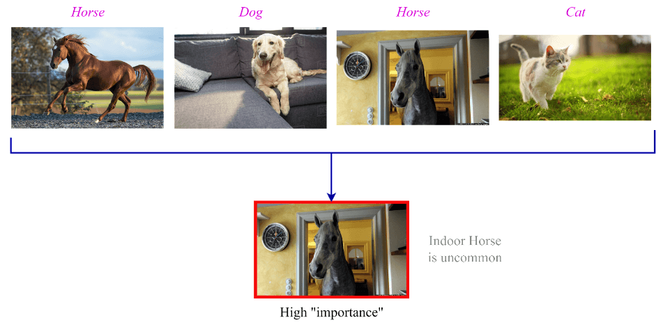
Reviewing the data samples, which obtained a very high “importance” value, can help identify potential labeling errors, which can then be corrected to rebuild the coreset. Viewing the important samples in the coreset is easily done using the following:
# Get the top “num_samples_to_view” most important samples from the class ‘horse’
result = service_obj.get_important_samples(
   		class_size={‘horse’: num_samples_to_view})
Now that you have identified the anomalous sample, you can either update their labels or remove them completely to make the coreset more reliable. You can do this easily using the following code.
#Update labels of some anomalous samples to be the ‘Dog’ class
service_obj.update_targets(indices, y=[‘Dog’] * len(indices))

#Removing the samples indices stored in the array `idxes_to_delete` from the Coreset
service_obj.remove_samples(indices=idxes_to_delete)
Follow these detailed articles to find and fix labels in image classification, object detection, semantic segmentation and NLP datasets.
Once you have fixed the sample labels or removed them, you can train your ML model on the coreset, and retrain it if necessary to optimize the model hyperparameters– all done in exponentially less time than having to deal with the whole dataset.
Conclusion
Anomaly detection can improve data quality by identifying errors and inconsistencies, improving data preprocessing, enhancing data validation, preventing fraud and misuse, and improving product and service quality. By leveraging anomaly detection techniques, organizations can gain insights into their data, prevent errors and fraud, and improve the accuracy and reliability of their data.
Whether you are working in finance, cybersecurity, manufacturing, or healthcare, anomaly detection is a crucial tool that can help you gain insights into your data and make better decisions. By staying up-to-date with the latest developments in anomaly detection, you can continue to improve your data analysis capabilities and gain a competitive edge in your respective industry.