
Machine learning models are at the heart of many applications and systems, from self-driving cars to recommendation engines to medical diagnosis. The performance and accuracy of these models heavily depend on how well they are trained. Model training involves feeding a dataset into a model, allowing it to learn from the data, and adjusting its parameters iteratively to optimize its performance. Efficient model training is crucial for achieving optimal model performance and reducing the development time of products.
In this blog, we will explore the intricacies of machine learning model training, including key concepts, challenges, and best practices for efficient training. Whether you are a beginner or an experienced practitioner in machine learning, this blog will provide valuable insights and actionable tips for enhancing your model training skills.
The Machine Learning Model Training Process
Machine learning (ML) model training teaches a computer (statistical) algorithm to recognize patterns in data and make predictions based on those patterns when novel data are presented. That is, we have a model with tunable parameters which need to be optimized based on the problem at hand, which we do by feeding it large amounts of data.
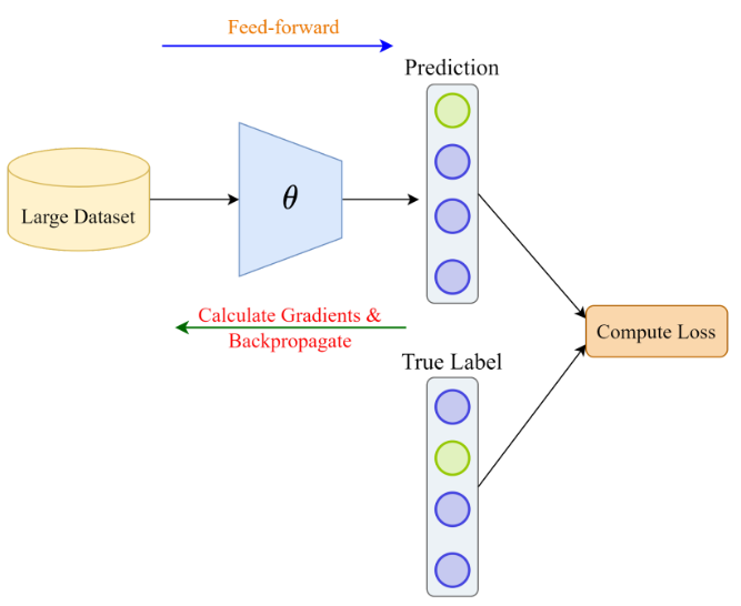
Deep Learning Model Training Pipeline
The accuracy and efficiency of a trained model depend on various factors, including data quality, model selection, hyperparameter tuning, regularization, evaluation, and deployment, the best practices for which we will discuss in the next section.
With the popularity of large Vision and/or Language Models- ChatGPT, GPT-4, Stable Diffusion, etc., the training time increases exponentially due to the models’ complex architecture and the training data volume. Coresets give a suitable alternative by creating a small, weighted subset of the original input dataset so that solving the problem on the Coreset will yield the same solution as solving the problem on the original big data, thus reducing your carbon footprint.
For more reasons to use Coresets, check out this video.
You can use the DataHeroes library to build a Coreset seamlessly and preserve model quality, as exemplified here, using which tuning hyperparameters for your model becomes much faster during the production pipeline.
Best Practices for Machine Learning Model Training
Machine learning (ML) model training is an essential process for building accurate and effective models that can recognize patterns and make predictions based on input data. However, the process can be complex and time-consuming, requiring careful planning and execution to ensure the model performs accurately and efficiently.
Data Preparation
The first step in training an ML model is data preparation. The quality of the training data significantly impacts the performance of the model. Therefore, it is essential to have high-quality, well-prepared training data that accurately represent the problem domain.
The data should be cleaned, pre-processed, and transformed to make it suitable for the model since data bias and imbalance can significantly affect its performance, leading to incorrect predictions. Here are some best practices for data preparation:
- Collect a representative dataset that covers all possible scenarios.
- Remove any errors, inconsistencies, or missing/duplicate values from the data.
- Transform the data into a format the model can understand, such as normalizing or standardizing the data.
Learn more about 5 Data Cleaning Techniques for Better ML Models.
Hyperparameter Tuning
Hyperparameters are the configuration settings of an ML model that are set before training, such as the learning rate, batch size, and regularization parameters. These hyperparameters significantly affect the model’s performance and should be carefully selected to achieve the best results.
Hyperparameter tuning is selecting the optimal hyperparameters for the model and problem. This can be a time-consuming and iterative process, but it is critical to the model’s success. Several techniques for hyperparameter tuning include grid search, random search, and Bayesian optimization.
Grid search involves exhaustively searching a predefined range of hyperparameters, while random search selects hyperparameters randomly from a predefined range. Bayesian optimization uses probabilistic models to predict the performance of different hyperparameters and selects the most promising ones for evaluation.
An example of tuning hyperparameters using Grid Search is shown below for a Support Vector Machines Classifier.
```
from sklearn.model_selection import GridSearchCV
from sklearn.svm import SVC
from sklearn.datasets import load_iris

# Load the dataset
iris = load_iris()

# Split the dataset into features (X) and target (y)
X = iris.data
y = iris.target

# Define the hyperparameters and their possible values
param_grid = {
    'C': [0.1, 1, 10],
    'kernel': ['linear', 'rbf', 'sigmoid'],
    'gamma': [0.1, 1, 'scale']
}

# Create an instance of the model
svm = SVC()

# Perform grid search cross validation
grid_search = GridSearchCV(svm, param_grid, cv=5)
grid_search.fit(X, y)

# Print the best hyperparameters and their corresponding score
print("Best Hyperparameters: ", grid_search.best_params_)
print("Best Score: ", grid_search.best_score_)
```
Using grid search is the most comprehensive approach for hyperparameter tuning, but it requires a lot of computational resources. However, performing grid search on a Coreset accelerates the process significantly (since a much smaller number of representative samples comprise the Coreset) and can be performed many times very fast, if needed, after data cleaning iterations. You can achieve this using the following code.
```
from dataheroes import CoresetTreeServiceLG
service_obj = CoresetTreeServiceLG.load(out_dir, save_tree_name)
coreset = service_obj.get_coreset() indices_coreset, X_coreset, y_coreset = coreset['data'] gs.fit(X_coreset, y_coreset, sample_weight=coreset['w'])
```
Choosing the Right Model
Selecting the right ML model for the problem at hand is crucial for achieving good results. Several types of ML models exist, including linear regression, logistic regression, decision trees, random forests, and neural networks. Each model has its strengths and weaknesses, and the choice of the model depends on the problem’s characteristics.
For example, if the problem is to predict a continuous value, linear regression or a neural network with a single output neuron may be suitable. If the problem is to classify data into two classes, logistic regression or a neural network with a single output neuron and a sigmoid activation function may be appropriate. If the problem is to classify data into multiple classes, a decision tree, random forest, or neural network with multiple output neurons and a softmax activation function may be useful.
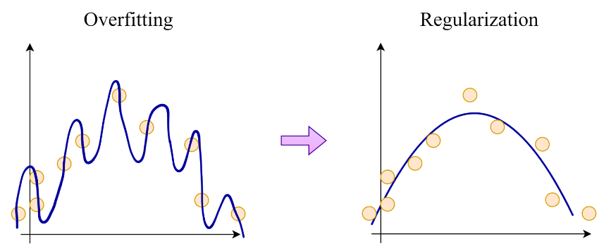
Model Regularization
ML models are prone to overfitting, i.e., the model performs exceptionally well on the training data by memorizing its patterns but cannot extend its knowledge to the test data (An example is shown below). Regularization is a technique that prevents overfitting by adding a penalty term to the model’s loss function that discourages large weights.
There are several types of regularization, including L1 regularization, L2 regularization, and dropout.
- L1 regularization adds a penalty proportional to the absolute value of the weights, encouraging sparsity.
- L2 regularization adds a penalty proportional to the square of the weights, encouraging small weights.
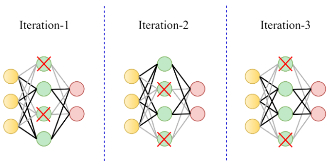
- Dropout randomly drops out a fraction of the neurons in a deep neural network during training, preventing the model from relying too much on any single neuron. During testing, all the neurons are used.

A code snippet showing L1 and L2 regularization in PyTorch is as follows.
```
import torch
import torch.nn as nn

# Define a custom model class
class MyModel(nn.Module):
    def __init__(self):
        super(MyModel, self).__init__()
        self.fc1 = nn.Linear(64, 32)
        self.fc2 = nn.Linear(32, 10)

    def forward(self, x):
        x = torch.relu(self.fc1(x))
        x = self.fc2(x)
        return x

# Create an instance of the custom model
model = MyModel()

# Define the L1 regularization strength
l1_strength = 0.01

# Define the L2 regularization strength
l2_strength = 0.01

# Define the loss function with regularization
criterion = nn.CrossEntropyLoss()
optimizer = torch.optim.Adam(model.parameters(), lr=0.001, weight_decay=l2_strength)

# Loop through each epoch of training
for epoch in range(num_epochs):
    # Forward pass
    outputs = model(inputs)
    loss = criterion(outputs, targets)

    # Apply L1 regularization to the loss
    if l1_strength > 0:
        l1_norm = torch.tensor(0.0)
        for param in model.parameters():
            l1_norm += torch.norm(param, p=1)
        loss += l1_strength * l1_norm

    # Backward pass and optimization
    optimizer.zero_grad()
    loss.backward()
    optimizer.step()

    # Print the loss for this epoch
    print('Epoch [{}/{}], Loss: {:.4f}'.format(epoch+1, num_epochs, loss.item()))
```
Dealing with Exploding/Vanishing Gradients
Vanishing and exploding gradients are common problems that occur during the training of deep neural networks. These issues can lead to slow convergence, unstable training, and poor model performance. In this section, we will discuss the causes of vanishing and exploding gradients and the techniques used to deal with them.
Vanishing Gradients
Vanishing gradients occur when the parameter gradients become too small during backpropagation, making it difficult for the network to learn. This problem is more common when a very deep neural network (models with many layers) is used on data that is not complex enough. The causes of vanishing gradients are:
- Activation Functions: Some activation functions, such as sigmoid and hyperbolic tangent (tanh), have a derivative that tends towards zero as the input becomes large or small. This means that the gradients of the layers that use these activation functions also become small, making it difficult for the network to learn.
- Initialization: The weights of the neural network are usually initialized randomly, and if the weights are too small, the gradients may also become too small during training.
- Deep Network Architecture: In deep networks, gradients are propagated through many layers, and each layer can amplify or dampen the gradients. If the amplification is weaker than the damping, the gradients will vanish.
Techniques to Deal with Vanishing Gradients:
- Activation Functions: ReLU (rectified linear unit) activation function is widely used in deep neural networks. Unlike sigmoid and tanh, the derivative of ReLU is always 1 or 0, which prevents the gradients from becoming too small.
- Initialization: The initialization of weights can be done using techniques such as Xavier or He initialization. These techniques help set the weights at a reasonable scale, reducing the risk of vanishing gradients.
- Network Architecture: Residual and skip connections have been shown to be effective in dealing with vanishing gradients. These connections allow the gradients to flow directly from one layer to another without being attenuated, thus reducing the risk of vanishing gradients.
An example code snippet in PyTorch is shown below to demonstrate how to perform Xavier initialization for weights and biases and use different activation functions like ReLU and tanh.
```
import torch
import torch.nn as nn
import torch.nn.init as init

# Define your custom neural network class
class MyNet(nn.Module):
    def __init__(self):
        super(MyNet, self).__init__()
        self.fc1 = nn.Linear(in_features=10, out_features=20)  # Input features: 10, Output features: 20
        self.fc2 = nn.Linear(in_features=20, out_features=5)   # Input features: 20, Output features: 5

        # Xavier initialization for weights and biases
        init.xavier_uniform_(self.fc1.weight)
        init.xavier_uniform_(self.fc1.bias)
        init.xavier_uniform_(self.fc2.weight)
        init.xavier_uniform_(self.fc2.bias)

    def forward(self, x):
        x = torch.relu(self.fc1(x))  # ReLU activation function
        x = torch.tanh(self.fc2(x))  # tanh activation function
        return x

# Instantiate your custom neural network
model = MyNet()

# Define your input data tensor
X = torch.randn(32, 10)  # Example input data of shape (batch_size, input_size)

# Forward pass to obtain predictions
predictions = model(X)

# Print the shape of the predictions tensor
print("Predictions shape: ", predictions.shape)
```
Exploding Gradients
Exploding gradients occur when the gradients become too large during backpropagation. This problem is also more common in deep neural networks with many layers. The causes of exploding gradients are:
- High Learning Rate: A high learning rate can cause the gradients to become too large, making it difficult for the network to learn.
- Poorly Designed Network Architecture: Poorly designed network architecture can cause the gradients to become too large.
Techniques to Deal with Exploding Gradients:
- Gradient Clipping: Gradient clipping is a technique used to limit the magnitude of the gradients during backpropagation. This prevents the gradients from becoming too large and stabilizes the training process.
- Lower Learning Rate: A lower learning rate can help prevent the gradients from becoming too large. However, a lower learning rate may also slow down the training process.
- Batch Normalization: Batch normalization is a technique that normalizes the inputs to each layer of the network. This helps stabilize the gradients and prevent them from becoming too large.
An example of using gradient clipping in PyTorch is as follows:
```
import torch
import torch.nn as nn
import torch.optim as optim

# Define your neural network model
class MyModel(nn.Module):
    def __init__(self):
        super(MyModel, self).__init__()
        self.fc1 = nn.Linear(100, 50)
        self.fc2 = nn.Linear(50, 10)

    def forward(self, x):
        x = torch.relu(self.fc1(x))
        x = self.fc2(x)
        return x

# Instantiate your model
model = MyModel()

# Define your loss function and optimizer
criterion = nn.CrossEntropyLoss()
optimizer = optim.SGD(model.parameters(), lr=0.01)

# Define your input data and target labels
inputs = torch.randn(32, 100)  # Example input data of shape (batch_size, input_size)
targets = torch.randint(0, 10, (32,))  # Example target labels of shape (batch_size,)

# Zero the gradients
optimizer.zero_grad()

# Forward pass
outputs = model(inputs)

# Compute the loss
loss = criterion(outputs, targets)

# Backward pass
loss.backward()

# Clip gradients to a maximum value
torch.nn.utils.clip_grad_norm_(model.parameters(), max_norm=1.0)

# Update the model weights
optimizer.step()
```
Model Evaluation
After training the model, it is essential to evaluate its performance to ensure that it is accurate and reliable and to compare it with other methods in a standard fashion. The evaluation should be performed on a separate subset of the training dataset that the model has not seen during training or hyperparameter tuning. This dataset is called the validation dataset, and it should be representative of the problem domain.
The most commonly used metrics for evaluating ML models are accuracy, precision, recall, F1 score, and AUC-ROC. Accuracy measures the percentage of correctly classified instances. For a binary class problem (with positive and negative classes), precision measures the proportion of correctly classified positive instances, recall measures the proportion of actual positive instances that were correctly classified, and the F1 score is the harmonic mean of precision and recall. AUC-ROC is the area under the receiver operating characteristic curve and measures the model’s ability to distinguish between positive and negative instances.
It is also essential to analyze the model’s performance on different subsets of the validation dataset to ensure that it performs well in all possible scenarios by a process called cross-validation. For example, if the problem involves classifying images of different types of animals, the model’s performance should be evaluated separately for each animal category. A code snippet for cross-validation is as follows.
```
from sklearn.model_selection import cross_val_score
from sklearn.model_selection import KFold
from sklearn.linear_model import LinearRegression

# Load your dataset
X, y = load_your_dataset()

# Create a linear regression model
model = LinearRegression()

# Define the number of folds for cross-validation
num_folds = 5

# Create a KFold object for cross-validation
kf = KFold(n_splits=num_folds, shuffle=True, random_state=42)

# Perform cross-validation and get scores
scores = cross_val_score(model, X, y, cv=kf)

# Print the mean and standard deviation of the scores
print("Cross-validation scores: ", scores)
print("Mean cross-validation score: ", scores.mean())
print("Standard deviation of cross-validation scores: ", scores.std())
```
Model Deployment
Once the model has been trained and evaluated, it is ready for deployment. The deployment process involves integrating the model into the production environment, where it can be used to make predictions on new data. The deployment process should be carefully planned and tested to ensure that the model works as expected and does not cause any disruptions to the production system.
It is essential to monitor the model’s performance in the production environment to ensure that it continues to perform well and that any issues are identified and addressed promptly. Monitoring can be done using various techniques, including logging, alerts, and dashboards.
Model Training using Coresets
Model training using Coresets is a relatively new and powerful machine learning approach that can dramatically reduce the computational cost and improve the efficiency of the model training process. Coresets-based Machine Learning involves selecting a small subset of the data that can accurately represent the entire data set and then training the machine learning model on the Coreset data.
- The DataHeroes Coreset library enables you to remove a noisy data sample or update its label for retraining the Coreset in O(1) order, allowing several clean-train iterations to ensue in a very short time.
- Also, since the Coreset training is many times faster than using the full dataset, several different models can be quickly tried out to select the optimal architecture for the problem at hand.
- If the Coreset performance is not satisfactory, the Coreset sample size can be expanded, and the model can be retrained on the updated Coreset without having to retrain on the entire dataset.
- Hyperparameter tuning is a significantly less cumbersome process since grid search can be applied on the Coresets very fast.
We only need a couple of lines of code to build the Coreset of a dataset using the DataHeroes library. An example is shown below for a dataset stored in a CSV file.
```
from dataheroes import CoresetTreeServiceLG
service_obj = CoresetTreeServiceLG(data_params=data_params,
                                   optimized_for='training',
                                   n_classes=7,
                                   n_instances=406_000
                                  )
service_obj.build_from_file(train_file_path)
```
Now to get the Coreset from your dataset, use the following code.
```
# Get the top level coreset (~2K samples with weights)
coreset = service_obj.get_coreset()
indices, X, y = coreset['data']
w = coreset['w']
# Train a logistic regression model on the coreset.
coreset_model = LogisticRegression().fit(X, y, sample_weight=w)
n_samples_coreset = len(y)
```
Finally, to use this coreset to train a model, say a Logistic Regression model, you can simply do the following.
```
X = train_file.iloc[:, :-1].to_numpy()
y = train_file.iloc[:, -1].to_numpy()

full_dataset_model = LogisticRegression().fit(X, y)
n_samples_full = len(y)
```
To follow a more in-depth step-by-step Python tutorial for building your own Coreset for model training, follow this easy GitHub documentation.
While training your models, you may also identify errors in your data, which you can quickly fix by using the following code.
```
indices, importance = service_obj.get_important_samples(class_size={‘non_defect’: 50}) service_obj.update_targets(indices, y=[‘defect’] * len(indices))
```
Final Thoughts
Training an ML model is a complex process that requires expertise and experience. This blog discussed the best practices and techniques for efficient ML model training. These include data preparation, hyperparameter tuning, choosing a suitable model, model regularization, model evaluation, and model deployment.
Following these practices ensures that the trained model is accurate, reliable, and scalable. However, it is essential to note that there is no one-size-fits-all approach to ML model training, and the best practices and techniques may vary depending on the problem domain and the data.
Therefore, it is important to continuously learn and adapt to new techniques and technologies and experiment with different approaches to find the best solution for each specific problem.