
Machine learning models have become ubiquitous in many areas of our lives, from predicting the weather to recommending products on e-commerce websites. However, building an effective machine learning model requires more than just choosing the right algorithm and feeding it data.
One of the most critical steps in the machine learning workflow is model tuning, which involves selecting the right hyperparameters and optimizing the model to achieve the best performance. Model tuning can be a challenging and time-consuming process, but it is essential for achieving the best possible results from your machine learning models.
What is Model Tuning?
Model tuning is the process of adjusting the hyperparameters of a Machine Learning model to achieve better performance. Hyperparameters are parameters that cannot be learned from the training data but need to be manually set by the user. Examples of hyperparameters include the learning rate, the number of hidden layers in a neural network, and the regularization parameter.
Effective model tuning is critical because it can significantly impact the accuracy and generalization performance of the model. By selecting the right hyperparameters, you can achieve better accuracy, reduce overfitting, and even make it more robust to data drift.
Model tuning is an iterative process that requires careful evaluation of the model’s performance on a validation set. By following best practices and strategies for model tuning, you can achieve better performance and improve the accuracy of your machine learning models.
How do you tune a model?
To tune a machine learning (ML) model, we must adjust its hyperparameters to optimize its performance on a given task. We start by choosing an appropriate evaluation metric and splitting the data into training and validation sets. Then, we select the hyperparameters we want to tune, define a search space, and choose an algorithm to explore that space efficiently.
We train and evaluate the model on the validation set using the chosen evaluation metric and repeat the process until we find the optimal hyperparameters. Finally, we test the model on a held-out test set to evaluate its performance on unseen data. The goal is to find the best set of hyperparameters that optimize the model’s performance while minimizing the computational resources required.
Manual and automated tuning are two approaches to tuning an ML model. Here are some key differences between these two approaches:
Manual Tuning:
- Human expertise is required to select hyperparameters.
- Hyperparameters are selected based on intuition, trial and error, and experience.
- The tuning process is time-consuming and can be subjective.
- The model’s performance is highly dependent on the expertise of the person tuning it.
- It is suitable for small datasets or simple models.
Automated Tuning:
- Hyperparameters are selected automatically using an algorithm.
- The algorithm searches the hyperparameter space efficiently.
- The tuning process is faster and less subjective.
- The model’s performance is less dependent on human expertise.
- It is suitable for large datasets or complex models.
Overall, automated tuning is preferred over manual tuning, especially for large datasets or complex models, because it can save time and improve the model’s performance. However, manual tuning can still be helpful in some situations where the model is simple, or the dataset is small.
10 Tips for Model Tuning
Let us now look into 10 tips and best practices for effective model tuning in machine learning. We will cover a range of techniques, including data preprocessing, hyperparameter optimization, regularization, and model architecture.
Whether you are just starting with machine learning or have been working in the field for some time, these tips will help you to optimize your models and achieve better results on your specific problem.
1. Try different Initialization Strategies
Initialization refers to assigning initial values to the parameters of a model, such as the weights and biases of the neural network. If the initial values are too small or too large, the gradients during backpropagation may become too small or too large, respectively, which can result in slow convergence or divergence.
This can be especially problematic in deep neural networks, where the gradients can become vanishingly small or explode due to the chain rule of differentiation, making it challenging for the model to learn the underlying patterns in the data. Thus, choosing the right initialization strategy is important for model tuning.
Xavier (or Glorot uniform) initialization and He initialization are the two most popularly used strategies. The PyTorch code for it is shown below.
import torch.nn as nn
import torch.nn.init as init

class MyModel(nn.Module):
    def __init__(self):
        super(MyModel, self).__init__()
        self.fc1 = nn.Linear(784, 256)
        self.fc2 = nn.Linear(256, 10)

        # Use Xavier initialization
        init.xavier_uniform_(self.fc1.weight)
        init.constant_(self.fc1.bias, 0)

        # Use He initialization
        init.kaiming_uniform_(self.fc2.weight)
        init.constant_(self.fc2.bias, 0)

    def forward(self, x):
        x = self.fc1(x)
        x = F.relu(x)
        x = self.fc2(x)
        return x
2. Use Ensembles
Ensembling is a technique for model tuning that combines multiple models to achieve better performance than any individual model. The idea behind ensembling is that each model in the ensemble can capture different patterns or aspects of the data (complementary features), and by combining them, the ensemble can be more robust and accurate.
Ensembling can be especially effective for complex problems or when working with limited data. By using multiple models, the ensemble can avoid overfitting the training data and generalize better to unseen data. Ensembling can also provide a measure of uncertainty in the predictions, which can be useful in applications such as risk assessment.
Several ensemble strategies exist, like probability averaging, majority voting, bagging, boosting, etc. Let us look at how to perform majority voting using Python.
from sklearn.ensemble import VotingClassifier
from sklearn.linear_model import LogisticRegression
from sklearn.svm import SVC
from sklearn.tree import DecisionTreeClassifier
from sklearn.datasets import load_iris
from sklearn.model_selection import train_test_split

# Load the iris dataset
iris = load_iris()
X, y = iris.data, iris.target

# Split the data into training and testing sets
X_train, X_test, y_train, y_test = train_test_split(X, y, test_size=0.2, random_state=42)

# Define the individual models to be ensembled
logreg = LogisticRegression(max_iter=1000)
svm = SVC(kernel='linear', probability=True)
dtree = DecisionTreeClassifier()

# Define the ensemble model with 'hard' voting
voting_clf = VotingClassifier(estimators=[('lr', logreg), ('svm', svm), ('dt', dtree)], voting='hard')

# Fit the ensemble model to the training data
voting_clf.fit(X_train, y_train)

# Evaluate the ensemble model on the testing data
score = voting_clf.score(X_test, y_test)
print("Ensemble model accuracy: {:.2f}%".format(score * 100))
3. Use Cross-Validation
Cross-validation is a technique used to evaluate the performance of machine learning models by splitting the data into multiple subsets, called “folds,” and training and testing the model on different combinations of these subsets. The goal of cross-validation is to obtain an estimate of the model’s performance on unseen data and to select the best hyperparameters.
In Python, we can use the sklearn.model_selection module to perform cross-validation:
from sklearn.model_selection import KFold, cross_val_score

# define the number of folds
kfold = Kfold(n_splits=10, shuffle=True, random_state=42)

# perform cross-validation
scores = cross_val_score(model, X, y, cv=kfold)

# print the mean and standard deviation of the scores
print(“Accuracy: %0.2f (+/- %0.2f)” % (scores.mean(), scores.std() * 2))
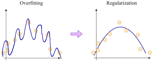
4. Use Regularization
Regularization is a technique used to prevent overfitting in machine learning models by adding a penalty term to the loss function. The penalty term encourages the model to have smaller weights or fewer non-zero coefficients, reducing the complexity of the model and making it more generalizable to new data.
We can use the sklearn.linear_model module to add regularization to linear regression models using L1 (Lasso) or L2 (Ridge) regularization.
From sklearn.linear_model import Lasso, Ridge

# define the Lasso regularization model
lasso = Lasso(alpha=0.1)

# define the Ridge regularization model
ridge = Ridge(alpha=0.1)

# fit the models to the training data
lasso.fit(X_train, y_train)
ridge.fit(X_train, y_train)

# evaluate the models on the test data
lasso_score = lasso.score(X_test, y_test)
ridge_score = ridge.score(X_test, y_test)

print(“Lasso score: “, lasso_score)
print(“Ridge score: “, ridge_score)
In PyTorch, we can add a weight decay parameter in the optimizer using the following code.
import torch
import torch.nn as nn
import torch.optim as optim

# define the neural network model
model = nn.Sequential(
    nn.Linear(10, 20),
    nn.ReLU(),
    nn.Linear(20, 1)
)

# define the optimizer with L2 regularization
optimizer = optim.Adam(model.parameters(), lr=0.001, weight_decay=0.01)

# train the model
for epoch in range(num_epochs):
    # forward pass
    outputs = model(inputs)
    loss = criterion(outputs, labels)

    # backward pass and optimization
    optimizer.zero_grad()
    loss.backward()
    optimizer.step()
5. Use Early Stopping
One of the techniques used for effective model tuning is early stopping. Early stopping refers to the technique of stopping the training of a model when its performance on a validation set stops improving. This is done to prevent overfitting, which occurs when a model learns the training data too well and becomes too specific to the training data, resulting in poor performance on new data.
Early stopping works by monitoring the model’s performance on a validation set during training. As the model is trained, its performance on the validation set is monitored regularly. If the performance of the model on the validation set does not improve for a certain number of consecutive epochs, training is stopped. The number of epochs after which training is stopped is determined by a parameter called “patience.”
import torch

# define your model architecture here
model = ...

# define your optimizer here
optimizer = ...

# define your loss function here
loss_fn = ...

# define your training and validation dataloaders here
train_dataloader = ...
val_dataloader = ...

# define the number of epochs to train for
num_epochs = ...

# initialize variables for tracking the best validation loss and the number of epochs since the last best validation loss
best_val_loss = float('inf')
epochs_since_best_val_loss = 0

# loop over the epochs
for epoch in range(num_epochs):
    # training loop
    for batch in train_dataloader:
        # zero the gradients
        optimizer.zero_grad()

        # forward pass
        output = model(batch)
        loss = loss_fn(output, batch['target'])

        # backward pass
        loss.backward()
        optimizer.step()

    # validation loop
    val_loss = 0
    with torch.no_grad():
        for batch in val_dataloader:
            output = model(batch)
            val_loss += loss_fn(output, batch['target']).item()

    val_loss /= len(val_dataloader)

    # check if the validation loss has improved
    if val_loss < best_val_loss:
        best_val_loss = val_loss
        epochs_since_best_val_loss = 0
        # save the model parameters
        torch.save(model.state_dict(), 'best_model.pt')
    else:
        epochs_since_best_val_loss += 1

    # check if early stopping criterion is met
    if epochs_since_best_val_loss >= patience:
        print('Validation loss has not improved in {} epochs. Training stopped.'.format(patience))
        break
6. Use Dropout
Dropout is a regularization technique that can be used to prevent overfitting in deep neural networks. In this technique, randomly selected neurons are dropped out during training, forcing the network to learn redundant representations of the data, which can improve the generalization performance of the model.
import torch
import torch.nn as nn
import torch.optim as optim

class Net(nn.Module):
    def __init__(self):
        super(Net, self).__init__()
        self.fc1 = nn.Linear(784, 512)
        self.dropout = nn.Dropout(p=0.5)
        self.fc2 = nn.Linear(512, 10)

    def forward(self, x):
        x = x.view(-1, 784)
        x = nn.functional.relu(self.fc1(x))
        x = self.dropout(x)
        x = self.fc2(x)
        return x

model = Net()
criterion = nn.CrossEntropyLoss()
optimizer = optim.SGD(model.parameters(), lr=0.01, momentum=0.5)

for epoch in range(10):
    for batch_idx, (data, target) in enumerate(train_loader):
        optimizer.zero_grad()
        output = model(data)
        loss = criterion(output, target)
        loss.backward()
        optimizer.step()
In this example, we add a Dropout layer with a probability of 0.5 after the first fully connected layer in our neural network, i.e., during training, half of the neurons in the first layer will be randomly dropped out.
7. Use Batch Normalization
Batch normalization is a technique used to improve the training of deep neural networks by normalizing the inputs of each layer. This can help to mitigate the problem of covariate shift, which occurs when the distribution of inputs to a layer changes during training. By normalizing the inputs, batch normalization can stabilize the distribution of activations throughout the network, making it easier to train.
Here is an example of using batch normalization in a PyTorch model:
import torch
import torch.nn as nn
import torch.optim as optim

class Net(nn.Module):
    def __init__(self):
        super(Net, self).__init__()
        self.fc1 = nn.Linear(784, 512)
        self.bn1 = nn.BatchNorm1d(512)
        self.fc2 = nn.Linear(512, 10)

    def forward(self, x):
        x = x.view(-1, 784)
        x = nn.functional.relu(self.bn1(self.fc1(x)))
        x = self.fc2(x)
        return x

model = Net()
criterion = nn.CrossEntropyLoss()
optimizer = optim.SGD(model.parameters(), lr=0.01, momentum=0.5)

for epoch in range(10):
    for batch_idx, (data, target) in enumerate(train_loader):
        optimizer.zero_grad()
        output = model(data)
        loss = criterion(output, target)
        loss.backward()
        optimizer.step()
8. Use a Learning Rate Scheduler
In machine learning, the learning rate is a hyperparameter that controls the step size of the optimizer during training. If the learning rate is too high, the optimizer may overshoot the optimal weights and fail to converge. If the learning rate is too low, the optimizer may take a long time to converge. To address this problem, we can use a learning rate scheduler, which adjusts the learning rate during training.
A learning rate scheduler is a function that maps the epoch number to a learning rate. In PyTorch, we can use the StepLR scheduler to decrease the learning rate after a certain number of epochs. For example, we can start with a high learning rate and decrease it by a factor of 0.1 every 10 epochs.
Here’s an example of using a learning rate scheduler in a PyTorch model:
import torch
import torch.nn as nn
import torch.optim as optim
from torch.optim.lr_scheduler import StepLR

class Net(nn.Module):
    def __init__(self):
        super(Net, self).__init__()
        self.fc1 = nn.Linear(784, 512)
        self.fc2 = nn.Linear(512, 10)

    def forward(self, x):
        x = x.view(-1, 784)
        x = nn.functional.relu(self.fc1(x))
        x = self.fc2(x)
        return x

model = Net()
criterion = nn.CrossEntropyLoss()
optimizer = optim.SGD(model.parameters(), lr=0.1, momentum=0.5)
scheduler = StepLR(optimizer, step_size=10, gamma=0.1)

for epoch in range(20):
    scheduler.step()
    for batch_idx, (data, target) in enumerate(train_loader):
        optimizer.zero_grad()
        output = model(data)
        loss = criterion(output, target)
        loss.backward()
        optimizer.step()
9. Optimize Hyperparameters
Hyperparameters are variables that are set before training a model and cannot be learned during training. They can significantly affect the model’s performance, and tuning them appropriately can boost its accuracy. Optimizing hyperparameters is an essential step in model tuning.
There are several approaches to optimize hyperparameters, such as Grid Search, Random Search, and Bayesian Optimization.
Grid Search, which is the most popular approach, involves creating a grid of all possible hyperparameter combinations and testing each combination to find the optimal one. Random Search is similar to Grid Search, but instead of creating a grid of all possible hyperparameter combinations, it randomly samples combinations from a defined search space. Here’s an example of a Random Search in Python:
from sklearn.model_selection import RandomizedSearchCV
from sklearn.ensemble import RandomForestClassifier
from scipy.stats import uniform

# Set up the parameter distribution
param_dist = {'n_estimators': [50, 100, 200], 'max_depth': [10, 20, 30], 'min_samples_split': [2, 5, 10],
              'min_samples_leaf': [1, 2, 4], 'bootstrap': [True, False], 'criterion': ['gini', 'entropy'],
              'max_features': ['sqrt', 'log2', None], 'class_weight': ['balanced', 'balanced_subsample']}

# Create a Random Forest object
rfc = RandomForestClassifier()

# Create Random Search Cross Validation object
random_search = RandomizedSearchCV(rfc, param_distributions=param_dist, n_iter=50, cv=5, random_state=42)

# Fit the random search object to the data
random_search.fit(X_train, y_train)

# Get the best hyperparameters
best_params = random_search.best_params_
Bayesian optimization is a more advanced technique that uses Bayesian inference to optimize hyperparameters. It builds a probabilistic model of the objective function and uses it to select the most promising hyperparameters to evaluate.
Here is an example code for Bayesian optimization using the scikit-optimize library in Python:
from skopt import BayesSearchCV
from sklearn.ensemble import RandomForestRegressor
from sklearn.datasets import load_boston
from sklearn.model_selection import train_test_split

# Load dataset
X, y = load_boston(return_X_y=True)

# Split the dataset into training and testing sets
X_train, X_test, y_train, y_test = train_test_split(X, y, test_size=0.2, random_state=42)

# Define the hyperparameter search space
search_space = {
    'n_estimators': (10, 100),
    'max_depth': (1, 20),
    'min_samples_split': (2, 20),
    'min_samples_leaf': (1, 20),
}

# Define the model and the search strategy
rf = RandomForestRegressor()
bayes = BayesSearchCV(
    estimator=rf,
    search_spaces=search_space,
    n_iter=50,
    cv=5,
    verbose=2,
    n_jobs=-1,
)

# Fit the model
bayes.fit(X_train, y_train)

# Evaluate the model
print(f"Best parameters: {bayes.best_params_}")
print(f"Training score: {bayes.best_score_:.3f}")
print(f"Testing score: {bayes.score(X_test, y_test):.3f}")
10. Use Coresets
Hyperparameter optimization requires retraining the model. When you have several hyperparameters, you may want to try different combinations of them. For models that take several days to train (due to model size or dataset size), it is infeasible to perform so many training passes from scratch to find the optimal parameters.
A Coreset is (usually) a small, weighted subset of the original input set of items, such that fitting an ML model on the Coreset will yield the same parameters as fitting it on the original big data. The DataHeroes Coreset tree structure allows you to re-train your model on the Coreset in near real-time, thus making it easy to try several different hyperparameter combinations.
Experiments on coresets show that even by reducing the dataset by 100 times, the test performance remains the same, as shown below.

Experiment with full dataset vs. Coreset. AUC=Area under (ROC) Curve
Coresets can lower your model update time down to minutes or hours and lower the costs significantly, thus making it practical to update your model as frequently as needed.
How to implement Coresets
In Python, the DataHeroes library can be easily installed using ‘pip install dataheroes’. Say you have a dataset consisting of 46,000,000 samples distributed in 7 classes. Although this is a medium-sized dataset in today’s information era, models can take several hours to fit the data based on its complexity.
To build a coreset on this 46M samples dataset, we only need a few lines of code:
from dataheroes import CoresetTreeServiceLG
service_obj = CoresetTreeServiceLG(data_params=data_params,
                                   optimized_for='training',
                                   n_classes=7,
                                   n_instances=46_000_000
                                  )
service_obj.build_from_file(train_file_path)
Now, suppose you want to fit a Logistic Regression model on this dataset; you can do the same on the coreset using the following code:
# Get the top level coreset (~20K samples with weights, in this case)
coreset = service_obj.get_coreset()
indices, X, y = coreset['data']
w = coreset['w']

# Now fit your model to the coreset
from sklearn.linear_model import LogisticRegression

coreset_model = LogisticRegression().fit(X, y, sample_weight=w)
To follow a more in-depth step-by-step Python tutorial for building your own Coreset for model training, follow this easy GitHub documentation.
A Logistic Regression classifier has three main hyperparameters which need to be set beforehand – the penalty type, the penalty/cost value, and the solver (however, all solvers don’t work with all penalty types). We can use the following code for a grid search approach on this coreset.
# Set up the parameter grid
param_grid = {'penalty': ['l1', 'l2'],
'C': [0.1, 1, 10, 100],
'Solver': ['liblinear','saga']
}

# Get the best hyperparameters (and optionally the model)
result = service_obj.grid_search(param_grid)
Now, using the best parameters of the Logistic Regression model, you can test the model on your test set.
Although hyperparameter tuning is vastly important for bringing out the optimal performance of the models, the training data must also be clean. Coresets can help with updating labels as well. Follow these detailed articles to find and fix labels in image classification, object detection, semantic segmentation, and NLP datasets.
For more tips on data cleaning to improve ML models, follow this article.
Conclusion
Model tuning is a critical step in machine learning that can have a significant impact on the performance and accuracy of our models. Following the 10 tips and best practices we outlined in this article, you can optimize your model and achieve better results on your specific problem.
However, model tuning can be an iterative and time-consuming process, and it may take several attempts to find the optimal combination of techniques and hyperparameters. Coresets help reduce this time and effort significantly through an intelligent subsample selection process. It is also crucial to have a solid understanding of the problem domain and the data we are working with to make informed decisions about which techniques and hyperparameters to use.