Comparing Coresets to Other Reduction and Sampling Techniques in Machine Learning

Machine learning algorithms often encounter large and complex datasets, leading to computational challenges and model performance issues. Reduction and sampling techniques are vital in overcoming these challenges by reducing dataset size and balancing class distributions. In this blog, we will delve into various types of reduction and sampling techniques in machine learning and understand their significance and then compare the accuracy between the models trained along with multiple techniques and the models trained on coreset data to check what is most suitable for our purpose when it comes to a large dataset.

Feature Reduction Techniques:

• Principal Component Analysis (PCA): Reduces high-dimensional datasets by identifying principal components that retain crucial information while reducing dimensionality.

Instance Reduction Techniques:

• Random Sampling: Selecting a subset of individuals/items from a population randomly, without any specific pattern or bias.
• Stratified Sampling: Dividing a population into homogeneous subgroups and selecting samples from each subgroup to ensure representation from all groups.

Why are they used?

• Reduce training time and address memory constraints.
• Improve model generalization by removing redundant or noisy instances.

Sampling Techniques:

• Oversampling: Increases the number of instances in the minority class by generating synthetic examples or replicating existing ones (e.g., Random Oversampling, SMOTE, ADASYN).
• Undersampling: Decreases the number of instances in the majority class to balance class distribution (e.g., Random Undersampling, Cluster Centroids).
• Combination Techniques: Utilizes a mix of oversampling and undersampling strategies to balance class distribution (e.g., SMOTEENN, SMOTETomek).

Why are they used?

• Handle imbalanced datasets by addressing class imbalance problems.
• Improve model performance on minority classes and reduce bias towards majority classes.

Reduction and sampling techniques are crucial in machine learning to handle challenges with large datasets and class imbalances and improve model performance.

Here are the key takeaways:

• Feature reduction techniques streamline input features, improving model efficiency.
• Instance reduction techniques reduce computational and storage requirements by reducing the number of instances.
• Sampling techniques balance class distributions in imbalanced datasets, improving performance on minority classes.
• Popular feature reduction techniques include PCA, RFE, and SelectKBest.
• Random Sampling and K-Means Clustering are common instance reduction techniques.
• Tomek Links help improve class separability by identifying close pairs of instances from different classes.
• Oversampling generates synthetic examples or replicates existing ones in the minority class.
• Undersampling reduces instances in the majority class to balance class distribution.
• Combination techniques combine oversampling and undersampling methods.
• Understanding dataset characteristics is crucial for selecting appropriate techniques.
• Reduction and sampling techniques contribute to building robust machine-learning models by enhancing efficiency, addressing imbalances, and improving performance on minority classes.

Coresets

A coreset is a small subset of a large dataset that retains most of the important information in the original dataset. Coresets are often used in machine learning to reduce the time and space required to train and evaluate machine learning models.

Here are some of the benefits of using coresets in machine learning:

• Reduced training time
• Reduced memory requirements
• Improved accuracy
• Scalability
• Robustness

By employing these techniques, machine learning practitioners can effectively handle data challenges and optimize their models for better results.

XGBoost, a popular gradient-boosting framework, offers powerful tools for enhancing model accuracy. In this blog post, we will explore the significance key component: XGBClassifier. We will then delve into how leveraging coreset data can further improve the accuracy of our models.

XGBClassifier: Empowering Classification Tasks

XGBClassifier is a specialized class within the XGBoost library designed explicitly for classification problems. XGBoost, known for its excellent performance in both regression and classification tasks, employs an ensemble of decision trees to make accurate predictions. The XGBClassifier class harnesses this power specifically for classification tasks, making it a versatile and effective tool.

Using XGBClassifier, we can take advantage of various features and functionalities to enhance our classification models:

1. Gradient Boosting: XGBClassifier leverages the gradient boosting technique, which involves iteratively adding decision trees to refine the model’s predictions. This iterative approach allows the model to learn complex patterns and relationships within the data.
2. Regularization: XGBoost offers regularization techniques such as L1 and L2 regularization. These techniques help control the complexity of the model and prevent overfitting, improving generalization and robustness.
3. Imbalanced Class Handling: XGBClassifier provides options to address imbalanced class distributions, a common challenge in classification tasks. By assigning different weights to samples or using specialized tree construction algorithms, XGBClassifier enables us to handle imbalanced data effectively.

Let’s dive deeper into different ways of enhancing the model’s accuracy!

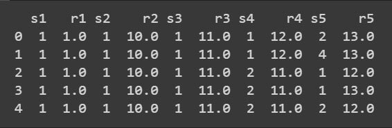
Dataset being used

Name: Pokerhand dataset

Size: 829201 Rows 11 Columns(including Index column)

Feature_names: [‘s1’, ‘r1’, ‘s2’, ‘r2’, ‘s3’, ‘r3’, ‘s4’, ‘r4’, ‘s5’, ‘r5’]

Target Name : ‘Class’

Top 5 rows of dataset

Why Pokerhand dataset?

• This dataset is suitable for multiclass classification because it has a reasonably large number of samples and ten distinct classes representing different poker hand types.
• Multiclass classification tasks involve predicting one class out of multiple possible classes, and the “pokerhand” dataset provides a good opportunity to apply and evaluate various multiclass classification algorithms and techniques.
• Moreover, the dataset’s features, representing the cards in a poker hand, are discrete and categorical, making it interesting for feature engineering and exploring techniques such as one-hot or ordinal encoding. It also offers a diverse range of potential patterns and dependencies to be learned by machine learning models.

Importing Necessary Libraries

import os
import warnings
from time import time

import numpy as np
import pandas as pd
import xgboost as xgb
from pathlib import Path

from sklearn.model_selection import train_test_split
from sklearn.datasets import fetch_openml
from sklearn.metrics import balanced_accuracy_score
from sklearn.preprocessing import StandardScaler, LabelEncoder, OneHotEncoder
from xgboost import XGBClassifier

from dataheroes import CoresetTreeServiceDTC

Dataset Preparation and function Definition

X, y = fetch_openml("pokerhand", return_X_y=True)

one_hot = OneHotEncoder(sparse=False)
one_hot.fit(X)
X = one_hot.transform(X)
X = X.astype(np.int8)

1. Load the PokerHand dataset from OpenML.
2. Create a new instance of the OneHotEncoder class.
3. Fit the encoder to the data.
4. Transform the data using the encoder.
5. All columns of the dataset, including numeric features, are one-hot encoded using OneHotEncoder from scikit-learn. The transformed X is stored back into X as a dense array.
6. Convert the data to the np.int8 data type.

label_enc = LabelEncoder()
y = label_enc.fit_transform(y)

Label Encoding: The target variable y is label-encoded using LabelEncoder from scikit-learn. This step is necessary because XGBoost requires consecutive integer labels starting from 0. The transformed y is stored back into y.

y[y > 3] = 4

Merge Class Labels: The code merges three class labels into a single label to reduce the number of targets from 10 to 5. This step is performed to avoid having imbalanced classes with a small number of samples for some classes.

# Apply standard scaling on the X.
scaler = StandardScaler()
X = scaler.fit_transform(X)

Standard Scaling: The features in X are standardized using StandardScaler from scikit-learn. This step scales the features to have zero mean and unit variance.

X_train, X_test, y_train, y_test = train_test_split(X, y, test_size=0.2, random_state=42)

num_classes = len(np.unique(y_train))
print(f"#classes={num_classes}, train size={len(X_train):,}, test size={len(X_test):,}")

n_estimators = 100

tree_query_level = 1
n_samples_full = len(y_train)

n_samples_rand_large = int(n_samples_full * 0.3)

def produce_results(experiment_group : str,
                    n_samp_full : int, n_samp_rand_large : int, n_samp_coreset : int,
                    full_score : float, rand_large_score : float, rand_csize_score : float, coreset_score : float,
                    full_secs : float, rand_large_secs : float, rand_csize_secs : float, coreset_secs : float):

    df = pd.DataFrame(data={
        ' ': ['Full dataset', 'Random bigger-sized sample', 'Random smaller-sized sample', 'Coreset'],
        'Training dataset size': [n_samp_full, n_samp_rand_large, n_samp_coreset, n_samp_coreset],
        '% of full dataset': [n_samp_full / n_samp_full, n_samp_rand_large / n_samp_full, n_samp_coreset / n_samp_full, n_samp_coreset / n_samp_full],
        'Balanced accuracy score': [full_score, rand_large_score, rand_csize_score, coreset_score],
        'Training time (sec)': [full_secs, rand_large_secs, rand_csize_secs, coreset_secs],
    })
    last_row = pd.IndexSlice[df.index[-1], :]
    styles = [dict(selector="caption", props=[("text-align", "center"), ("font-size", "120%"), ("font-weight", "bold")])]
    s  = df.style \
        .set_properties(subset=[' '],**{'text-align':'left'}) \
        .set_properties(subset=['Training dataset size','% of full dataset','Balanced accuracy score','Training time (sec)'],**{'text-align':'right'}) \
        .set_properties(subset=last_row, **{'color':'green', 'font-weight':'bold'}) \
        .set_caption(f"{experiment_group} Results") \
        .format({
        'Training dataset size': '{:,}',
        '% of full dataset': '{:.2%}',
        'Balanced accuracy score': '{:.4f}',
        'Training time (sec)': '{:.2f}'}) \
        .hide(axis='index') \
        .set_table_styles(styles)
    return s

This code performs several data preprocessing steps and defines functions for later summarizing the results. Let’s go through it step by step:

• Train-Test Split: The preprocessed data is split into training and testing sets using train_test_split from scikit-learn. The training set is assigned to X_train and y_train, while the testing set is assigned to X_test and y_test. The test size is set to 20% of the dataset, and the random state is fixed for reproducibility.
• Number of Classes: The number of classes is determined by finding the length of unique elements in y_train. It is stored in num_classes.
• Define Number of Estimators: The number of estimators for the XGBoost model is set to 100 and stored in n_estimators.
• Tree Query Level: The code defines the tree query level to 1, which means the tree node level at which the comparison is performed. It is stored in tree_query_level.
• Number of Samples: The total number of samples in the training set (X_train) is stored in n_samples_full.
• Define Number of Samples for Comparison: The number of samples for the random larger-sized sample and coreset is defined as a percentage of n_samples_full. The specific percentage used is 30%, and the values are stored in n_samples_rand_large and n_samples_coreset, respectively.
• Results Summary Function: A function named produce_results is defined to summarize the experimental results in a neat table. It takes various inputs such as dataset sizes, accuracy scores, and training times for different flavors of the experiment and returns a stylized Pandas DataFrame containing the summary table.

This code sets up the data preprocessing and summary functions required for the subsequent experimental analysis using XGBoost and coreset data.

Building the coreset

t = time()
service_obj = CoresetTreeServiceDTC(optimized_for='training',
                                    chunk_size=40_000,
                                    coreset_size=15_000)
service_obj.build(X_train, y_train)
coreset_build_secs = time() - t
print(f"Coreset build time (sec): {coreset_build_secs:.2f}")

• The first line, t = time(), starts a timer. This will be used to measure the amount of time it takes to build the coreset.
• The next few lines create a CoresetTreeServiceDTC object and call its build() method. This method will build the coreset from the training data.
• The next line, coreset_build_secs = time() – t, stops the timer and stores the difference in seconds.
• The last line, print(f”Coreset build time (sec): {coreset_build_secs:.2f}”), prints the coreset build time in seconds.

t = time()
# Get the coreset from the tree.
coreset = service_obj.get_coreset(level=tree_query_level)
indices_coreset_, X_coreset, y_coreset = coreset['data']
w_coreset = coreset['w']

# Train an XGBoost model on the coreset.
# For multiclass classification problems, the correct objective would be 'multi:softmax'.
xgbclassifier_coreset_model = XGBClassifier(objective='multi:softmax',
                                            num_class=num_classes,
                                            n_estimators=n_estimators)
xgbclassifier_coreset_model.fit(X_coreset, y_coreset, sample_weight=w_coreset)
n_samples_coreset = len(y_coreset)
xgbclassifier_coreset_secs = time() - t

• Starts a timer.
• Gets the coreset from the tree and stores it in a variable.
• Creates an XGBoost model with the specified parameters.
• Trains the XGBoost model on the coreset.
• Stores the number of samples in the coreset.
• Stops the timer and stores the difference in seconds.

t = time()
# Train an XGBoost model on the entire data-set.
xgbclassifier_full_model = XGBClassifier(objective='multi:softmax',
                                         num_class=num_classes,
                                         n_estimators=n_estimators)
xgbclassifier_full_model.fit(X_train, y_train)
xgbclassifier_full_secs = time() - t

• Starts a timer.
• Creates an XGBoost model with the specified parameters.
• Trains the XGBoost model on the entire dataset.
• Stops the timer and stores the difference in seconds.

These are the steps we will follow in mostly all the examples. Let’s move forward with Random Sampling first!

Random Sampling

t = time()
# Train an XGBoost model on the random data-set -
# (1) Create the model, (2) randomly sample the exact size as the coreset size, and (3) train the model.
xgbclassifier_rand_csize_model = XGBClassifier(objective='multi:softmax',
                                               num_class=num_classes,
                                               n_estimators=n_estimators)
xgbclassifier_rand_csize_idxs = np.random.choice(n_samples_full, n_samples_coreset, replace=False)
xgbclassifier_rand_csize_model.fit(X_train[xgbclassifier_rand_csize_idxs, :], y_train[xgbclassifier_rand_csize_idxs])
xgbclassifier_rand_csize_secs = time() - t

1. Create an XGBoost model with the specified parameters.
2. Randomly sample a subset of the training data the same size as the coreset.
3. Train the XGBoost model on the randomly sampled data.

The first step in the code snippet is to create an XGBoost model with the specified parameters. The XGBClassifier() function is used to create the model. The objective parameter is set to multi:softmax to indicate that the model should be trained for multi-class classification. The num_class parameter is set to the number of classes in the dataset. The n_estimators parameter is set to the number of trees that should be built in the model.

The second step in the code snippet is to randomly sample a subset of the training data that is the same size as the coreset. The np.random.choice() function is used to draw the samples without replacement. The n_samples_full variable is used to specify the population size from which the samples are drawn. The n_samples_coreset variable is used to specify the number of samples that should be drawn.

The third step in the code snippet is to train the XGBoost model on the randomly sampled data. The fit() method is used to train the model. The X_train[xgbclassifier_rand_csize_idxs, :] and y_train[xgbclassifier_rand_csize_idxs] arguments specify the training data and labels, respectively.The code snippet then stores the training time in the xgbclassifier_rand_csize_secs variable. This variable can then be used to compare the training time of the coreset model to the training time of a model that is trained on a randomly sampled dataset that is the same size as the coreset.

Training model on large Random Dataset

t = time()
# Train an XGBoost model on the random data-set -
# (1) Create the model, (2) randomly sample size larger than the coreset size, and (3) train the model.
xgbclassifier_rand_large_model = XGBClassifier(objective='multi:softmax',
                                               num_class=num_classes,
                                               n_estimators=n_estimators)
xgbclassifier_rand_large_idxs = np.random.choice(n_samples_full, n_samples_rand_large, replace=False)
xgbclassifier_rand_large_model.fit(X_train[xgbclassifier_rand_large_idxs, :], y_train[xgbclassifier_rand_large_idxs])
xgbclassifier_rand_large_secs = time() - t

1. Create an XGBoost model with the specified parameters.
2. Randomly sample a subset of the training data larger than the coreset.
3. Train the XGBoost model on the randomly sampled data.

The first step in the code snippet is to create an XGBoost model with the specified parameters. The XGBClassifier() function is used to create the model. The objective parameter is set to multi:softmax to indicate that the model should be trained for multi-class classification. The num_class parameter is set to the number of classes in the dataset. The n_estimators parameter is set to the number of trees that should be built in the model.

The second step in the code snippet is to randomly sample a subset of the training data that is larger than the coreset. The np.random.choice() function is used to draw the samples without replacement. The n_samples_full variable is used to specify the population size from which the samples are drawn. The n_samples_rand_large variable is used to specify the number of samples that should be drawn.

The third step in the code snippet is to train the XGBoost model on the randomly sampled data. The fit() method is used to train the model. The X_train[xgbclassifier_rand_large_idxs, :] and y_train[xgbclassifier_rand_large_idxs] arguments are used to specify the training data and labels, respectively.

The code snippet then stores the training time in the xgbclassifier_rand_large_secs variable. This variable can then be used to compare the training time of the coreset model to the training time of a model that is trained on a randomly sampled dataset that is larger than the coreset.

Model Evaluation

xgbclassifier_full_score = balanced_accuracy_score(y_test, xgbclassifier_full_model.predict(X_test))
xgbclassifier_rand_large_score = balanced_accuracy_score(y_test, xgbclassifier_rand_large_model.predict(X_test))
xgbclassifier_rand_csize_score = balanced_accuracy_score(y_test, xgbclassifier_rand_csize_model.predict(X_test))
xgbclassifier_coreset_score = balanced_accuracy_score(y_test, xgbclassifier_coreset_model.predict(X_test))
produce_results("XGBClassifier",
                n_samples_full, n_samples_rand_large, n_samples_coreset,
                xgbclassifier_full_score, xgbclassifier_rand_large_score, xgbclassifier_rand_csize_score, xgbclassifier_coreset_score,
                xgbclassifier_full_secs, xgbclassifier_rand_large_secs, xgbclassifier_rand_csize_secs, xgbclassifier_coreset_secs)

1. Calculate the balanced accuracy score for each model.
2. Call the produce_results() function to print the results of the evaluation.

The balanced_accuracy_score() function is used to calculate the balanced accuracy score for a model. The balanced accuracy score is a measure of accuracy that takes into account the class imbalance in the dataset.

The produce_results() function is used to print the results of the evaluation. The function takes the following arguments:

• The name of the model.
• The number of samples in the full dataset, the randomly sampled large dataset, and the coreset.
• The balanced accuracy scores for the full dataset, the randomly sampled large dataset, the randomly sampled coreset, and the coreset.
• The training times for the full dataset, the randomly sampled large dataset, the randomly sampled coreset, and the coreset.

The code snippet then prints the results of the evaluation. The results of the evaluation will show the balanced accuracy score and the training time for each model.

Stratified Sampling

t = time()
# Train an XGBoost model on the random data-set -
# (1) Create the model, (2) randomly sample the exact size as the coreset size, and (3) train the model.
xgbclassifier_strat_csize_model = XGBClassifier(objective='multi:softmax',
                                               num_class=num_classes,
                                               n_estimators=n_estimators)
xgbclassifier_strat_csize_idxs = np.array([], dtype=np.int64)

# Create a StratifiedShuffleSplit object for stratified sampling
sss = StratifiedShuffleSplit(n_splits=1, train_size=n_samples_coreset, random_state=42)

# Perform stratified sampling
for train_index, _ in sss.split(np.zeros(n_samples_full), y_train):
    xgbclassifier_strat_csize_idxs = train_index

# Shuffle the indexes to randomize the order
np.random.shuffle(xgbclassifier_strat_csize_idxs)
# xgbclassifier_rand_csize_idxs = np.random.choice(n_samples_full, n_samples_coreset, replace=False)
xgbclassifier_strat_csize_model.fit(X_train[xgbclassifier_strat_csize_idxs, :], y_train[xgbclassifier_strat_csize_idxs])
xgbclassifier_strat_csize_secs = time() - t

1. Create a StratifiedShuffleSplit object.
2. Use the StratifiedShuffleSplit object to perform stratified sampling.
3. Shuffle the indexes to randomize the order.
4. Train the XGBoost model on the stratified data.

The StratifiedShuffleSplit object is a class that is used to perform stratified sampling. The n_splits parameter is set to 1, which means that the data will be split into one train and test set. The train_size parameter is set to the size of the coreset. The random_state parameter is set to 42, which ensures that the results are reproducible.

The split() method of the StratifiedShuffleSplit object is used to perform stratified sampling. The split() method returns two arrays: a train index array and a test index array. The train index array contains the indices of the data points that were selected for the train set. The test index array contains the indices of the data points that were selected for the test set.

The shuffle() method of the np.random module is used to shuffle the indexes. This is done to randomize the order of the data points.

t = time()
# Train an XGBoost model on the random data-set -
# (1) Create the model, (2) randomly sample size larger than the coreset size, and (3) train the model.
xgbclassifier_strat_large_model = XGBClassifier(objective='multi:softmax',
                                               num_class=num_classes,
                                               n_estimators=n_estimators)
xgbclassifier_strat_large_idxs = np.array([], dtype=np.int64)
# Create a StratifiedShuffleSplit object for stratified sampling
sss = StratifiedShuffleSplit(n_splits=1, train_size=n_samples_strat_large, random_state=42)
# Perform stratified sampling
for train_index, _ in sss.split(np.zeros(n_samples_full), y_train):
    xgbclassifier_strat_large_idxs = train_index
# Shuffle the indexes to randomize the order
np.random.shuffle(xgbclassifier_strat_large_idxs)
xgbclassifier_strat_large_model.fit(X_train[xgbclassifier_strat_large_idxs, :], y_train[xgbclassifier_strat_large_idxs])
xgbclassifier_strat_large_secs = time() - t

The main difference between this code snippet and the previous code snippet is that the train_size parameter of the StratifiedShuffleSplit object is set to n_samples_strat_large instead of n_samples_coreset. This means that the stratified coreset will be larger than the original coreset.

Model Evaluation

# Evaluate models.
xgbclassifier_full_score = balanced_accuracy_score(y_test, xgbclassifier_full_model.predict(X_test))
xgbclassifier_strat_large_score = balanced_accuracy_score(y_test, xgbclassifier_strat_large_model.predict(X_test))
xgbclassifier_strat_csize_score = balanced_accuracy_score(y_test, xgbclassifier_strat_csize_model.predict(X_test))
xgbclassifier_coreset_score = balanced_accuracy_score(y_test, xgbclassifier_coreset_model.predict(X_test))
produce_results("XGBClassifier",
                n_samples_full, n_samples_strat_large, n_samples_coreset,
                xgbclassifier_full_score, xgbclassifier_strat_large_score, xgbclassifier_strat_csize_score, xgbclassifier_coreset_score,
                xgbclassifier_full_secs, xgbclassifier_strat_large_secs, xgbclassifier_strat_csize_secs, xgbclassifier_coreset_secs)

• Calculate the balanced accuracy score for each model.
• Call the produce_results() function to print the results of the evaluation.

Downsampling

Downsampling and training an XGBoost model

t = time()
# Calculate the number of samples to downsample
n_samples_downsample = n_samples_downsample_large
xgbclassifier_downsampled_large_model = XGBClassifier(objective='multi:softmax',
                                               num_class=num_classes,
                                               n_estimators=n_estimators)
# Get the number of samples in the training set
n_samples_full = len(X_train)

# Get the indexes for the majority class (class label 0)
majority_class_indexes = np.where(y_train == 0)[0]
minority_class_indexes = np.setdiff1d(np.arange(n_samples_full), majority_class_indexes)
# Perform downsampling of the majority class
downsampled_indexes = resample(majority_class_indexes, n_samples=n_samples_downsample, replace=False)

# Combine the indexes of the majority class with the indexes of the minority class
downsampled_indexes = np.concatenate((downsampled_indexes, minority_class_indexes))

# Shuffle the indexes to randomize the order
np.random.shuffle(downsampled_indexes)


xgbclassifier_downsampled_large_model.fit(X_train[downsampled_indexes, :], y_train[downsampled_indexes])
xgbclassifier_strat_large_secs = time() - t

1. Calculate the number of samples to downsample.
2. Create an XGBoost model.
3. Get the indexes for the majority class (class label 0).
4. Get the indexes for the minority class.
5. Perform downsampling of the majority class.
6. Combine the indexes of the majority class with those of the minority class.
7. Shuffle the indexes to randomize the order.
8. Use the downsampled indexes for further analysis.
9. Train the XGBoost model on the downsampled dataset.

The first step is to calculate the number of samples to downsample. This is done by setting the n_samples_downsample variable to the value of n_samples_downsample_large. The n_samples_downsample_large variable is a constant that is defined outside of the code snippet.

The second step is to create an XGBoost model. This is done by creating an instance of the XGBClassifier class and setting the objective parameter to multi:softmax. The multi:softmax objective function is used for multi-class classification problems.

The third step is to get the indexes for the majority class (class label 0). This is done using the np.where() function to find the indexes of all the data points in the training set with a class label of 0.

The fourth step is to get the indexes for the minority class. This is done by using the np.setdiff1d() function to find the indexes of all the data points in the training set that do not have a class label of 0.

The fifth step is to perform downsampling of the majority class. This is done by using the resample() function from the sklearn.utils module. The resample() function takes two arguments: the indexes of the majority class and the number of samples to downsample.

The replace=False parameter is used to ensure that the data points are not duplicated in the downsampled dataset.

The sixth step is to combine the indexes of the majority class with the indexes of the minority class. This is done by using the np.concatenate() function.

The seventh step is to shuffle the indexes to randomize the order. This is done by using the np.random.shuffle() function.

The eighth step is to use the downsampled indexes for further analysis. This is done by setting the X_downsampled and y_downsampled variables to the downsampled data and labels, respectively.

t = time()

# Calculate the number of samples to downsample from each class
n_samples_downsample_per_class = n_samples_coreset // 2

Explanation:

• n_samples_coreset is the desired size of the downsampled dataset, which should be equal to the size of the coreset (20,000 samples).
• n_samples_downsample_per_class is calculated by dividing n_samples_coreset by 2 using the floor division operator //. The purpose of this division is to ensure that we have an equal number of samples from both classes (class label 0 and other classes) in the downsampled dataset.

# Get the number of samples in the training set
n_samples_full = len(X_train)

# Get the indexes for the majority class (class label 0)
majority_class_indexes = np.where(y_train == 0)[0]
minority_class_indexes = np.setdiff1d(np.arange(n_samples_full), majority_class_indexes)

# Perform downsampling of both classes to match the size of the coreset
downsampled_majority_indexes = resample(majority_class_indexes, n_samples=n_samples_downsample_per_class, replace=False)
downsampled_minority_indexes = resample(minority_class_indexes, n_samples=n_samples_downsample_per_class, replace=False)

Explanation:

• n_samples_full is the total number of samples in the original training set (X_train).
• majority_class_indexes contains the indexes of samples belonging to the majority class, which is identified by class label 0.
• minority_class_indexes contains the indexes of samples belonging to the minority class (non-class label 0).
• The goal of downsampling is to create a balanced dataset with an equal number of samples from each class, matching the size of the coreset.

Note: The resample() function from sklearn.utils is used twice, once for the majority class and once for the minority class. It randomly selects samples without replacement from each class, ensuring that each class contributes the same number of samples to the downsampled dataset. The parameter replace=False ensures that samples are not duplicated during the downsampling process.

# Combine the indexes of the majority class with the indexes of the minority class

downsampled_indexes = np.concatenate((downsampled_majority_indexes, downsampled_minority_indexes))

# Shuffle the indexes to randomize the order
np.random.shuffle(downsampled_indexes)

# Use the downsampled indexes for further analysis
X_downsampled = X_train[downsampled_indexes]
y_downsampled = y_train[downsampled_indexes]

Explanation:

• downsampled_indexes is an array containing the combined indexes of the majority class and minority class after downsampling.
• np.concatenate() is used to combine the two sets of downsampled indexes into a single array.
• np.random.shuffle() shuffles the indexes randomly to ensure that the order of samples in the downsampled dataset is randomized.
• X_downsampled and y_downsampled are the downsampled feature matrix and target labels, respectively, which will be used for further analysis and modeling.

xgbclassifier_downsampled_csize_model = XGBClassifier(objective='multi:softmax',
                                                      num_class=num_classes,
                                                      n_estimators=n_estimators)

xgbclassifier_downsampled_csize_model.fit(X_downsampled, y_downsampled)

Explanation:

• xgbclassifier_downsampled_csize_model is an instance of the XGBoost classifier created with appropriate parameters for a multi-class classification problem.
• xgbclassifier_downsampled_csize_model.fit(X_downsampled, y_downsampled) fits the classifier on the downsampled data (X_downsampled and y_downsampled) to train the model.

Following the same steps as the previous snippet, just the number of data we are taking is less than the previous snippet.

Model Evaluation

xgbclassifier_full_score = balanced_accuracy_score(y_test, xgbclassifier_full_model.predict(X_test))
xgbclassifier_downsampled_large_score = balanced_accuracy_score(y_test, xgbclassifier_downsampled_large_model.predict(X_test))
xgbclassifier_downsampled_csize_score = balanced_accuracy_score(y_test, xgbclassifier_downsampled_csize_model.predict(X_test))
xgbclassifier_coreset_score = balanced_accuracy_score(y_test, xgbclassifier_coreset_model.predict(X_test))
produce_results("XGBClassifier",
                n_samples_full, n_samples_strat_large, n_samples_coreset,
                xgbclassifier_full_score, xgbclassifier_downsampled_large_score, xgbclassifier_downsampled_csize_score, xgbclassifier_coreset_score,
                xgbclassifier_full_secs, xgbclassifier_strat_large_secs, xgbclassifier_downsampled_csize_secs, xgbclassifier_coreset_secs)

• Calculate the balanced accuracy score for each model.
• Call the produce_results() function to print the results of the evaluation.

Conclusion

Data	Training dataset Size	% of full dataset	Balanced Accuracy Score	Training time (sec)
Full dataset	663,360	100.00%	0.9723	1366.27
Random bigger-sized sample	199,008	30.00%	0.9508	368.09
Random smaller-sized sample	20,883	3.15%	0.8273	37.35
Stratified bigger-sized sample	199,008	30.00%	0.9598	358.46
Stratified smaller-sized sample	20,854	3.14%	0.8191	37.49
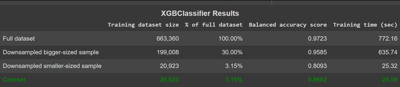
Downsample bigger-sized sample	199,008	30.00%	0.9585	635.74
Downsample smaller-sized sample	20,923	3.15%	0.8093	25.32
Coreset	20,923	3.15%	0.9602	24.59

• Coresets are a recent development in machine learning, but they have already been shown to be effective in a variety of applications.
• There are several reasons why coresets are better than other techniques for training machine learning models. First, coresets can significantly reduce the training time by training the model on a smaller subset of the data. This is especially important for large datasets, where training a model on the entire dataset can be time-consuming and expensive.
• Coresets can reduce memory requirements by storing the coreset instead of the entire dataset. This can be important for machine learning models that require a lot of memory to store.
• Coresets can improve the accuracy of machine learning models. This is because coresets are designed to retain the most important information in the original dataset. As a result, models trained on coresets are often more accurate than models trained on the entire dataset.
• Finally, coresets are scalable and robust. This means they can be used to train machine learning models on large and complex datasets.
• Overall, coresets are powerful tools that can improve the performance of machine learning models. They are especially useful for large datasets and for problems where the data is very high-dimensional.